
How do you tackle the Tail Problem in a Capital Model
In our fourth and final blog on the topic of challenging risk models, Tony and John look at the tail problem associated with different distribution models. Operational Risk Software can be key to supporting this discipline.
Taken from: Mastering Risk Management
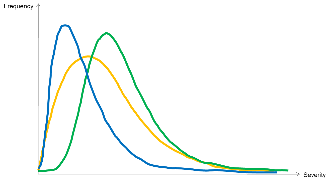
As noted in our previous blog (Link: Guide to parameters for challenging the Economic Capital Model) different distributions have different sizes of tails. Some distributions have thin tails and other fat tails. The term thin or fat refers to the right-hand end of the curve of the distribution in the area where large severities are recorded. A distribution with a fat tail will record a higher frequency for the same severity than a distribution with a thin tail.
In the diagram below, the Gumbel has the fattest tail; with the Weibull in the middle and the Lognormal with the thinnest tail. With this set of distributions Gumbel would be likely to give the highest capital value as it has the highest frequency for a particular severity.
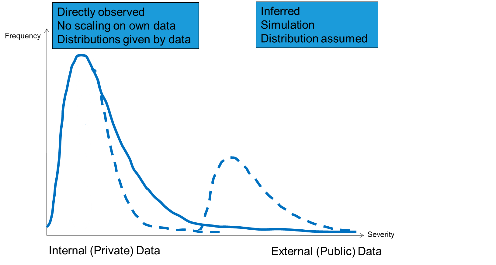
However, the tail problem does not stop there. There is a more general problem with the tails of all distributions in that they all appear to be not fat enough (i.e. not a high enough frequency for a given severity). Consider the number of major events that have occurred in recent years and that include USB, Societe Generale, Kidder Peabody, LTCM, Barings, JPMorgan Chase and a considerable number of others. The frequency for events of this size is much higher than that predicted by any of the distributions. This means that something else is happening at the right-hand end of the curve.
The diagram below solves the problem posed above by suggesting that there is another distribution (the dotted line) at the right-hand end of the curve which is not taken into account by single distribution modelling. Some advanced modellers create an additional distribution at the extreme right-hand end of the curve in order to account for the much higher frequency of events than could be expected from a single distribution. It is very difficult to model this second distribution as by definition there are even fewer data points. However, a relatively easy way around the problem is simply to take the answer given by the single distribution and multiply by a fixed factor, say, three or four.
The above two points on tails of distributions illustrate that modelling is not an exact science and only gives you an approximate answer from which to start further analysis. Modelling should never be seen as a solution in its own right but rather as another step along the path to an appropriate value for economic capital.
Summary
There are many ways to affect the capital calculation and these should all be challenged by an appropriate body, such as the risk committee. Some firms however have a specialist committee (often called the ‘model validation committee) which is staffed by modelling specialists as well as business line and risk people. It is important that the modellers are challenged and that they do not prevail simply because they using technical jargon.
In our next blog series Tony and John discuss the importance of risk management reporting.
Mastering Risk Management by Tony Blunden and John Thirlwell is published by FT International. Order your copy here: https://www.pearson.com/en-gb/subject-catalog/p/mastering-risk-management/P200000003761/9781292331317
For more information about how Operational Risk software can help your organisation, contact us today on sales@risklogix-solutions.com